By Christophe Blot

In March 2022, the US central bank began tightening monetary policy in response to rapidly rising inflation. Since then, the target rate for monetary policy has been increased at each meeting of the Federal Open Market Committee (FOMC), and now stands at 5%. The aim of these decisions is to bring inflation back towards the Federal Reserve’s 2% target. After peaking in the summer of 2022, inflation has fallen in line with the fall in energy prices. Thus far, economic activity has been resilient, and the unemployment rate has remained stable despite the tighter monetary and financial conditions. Will inflation continue to fall, and, more importantly, can it converge on the target without pushing up unemployment?

Inflation under control?

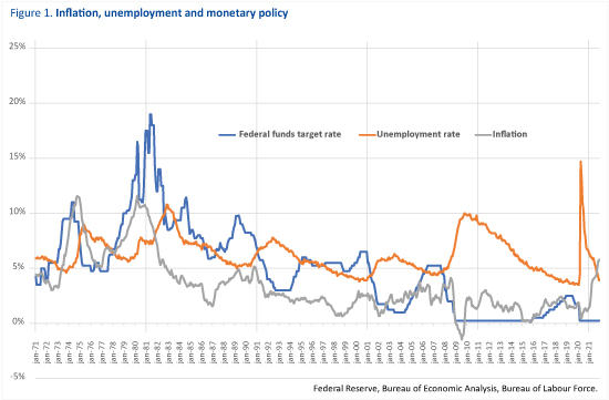
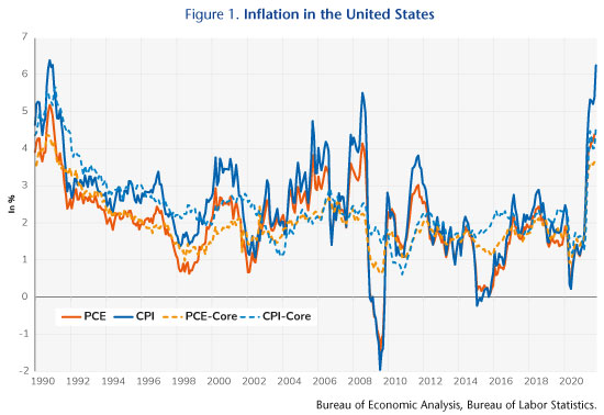
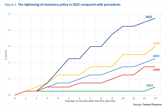
The Federal Reserve had been cautious throughout 2021, under the view that the increase in prices would be transitory. It was not until March 2022 that it began tightening, just over a year after inflation began to rise above the 2% target, when it had reached 6.8%[1]. The rise in prices has in fact proved to be more prolonged than FOMC members had anticipated and has spread to all components of the index. Finally, the central bank also feared the risk of a disconnection in inflation expectations, which would have sustained an inflationary spiral. Once it began to act, rate hikes occurred in rapid succession, with the target rate for federal funds rising from 0.25% to 5% in one year, i.e. a much faster pace of tightening than that observed in previous cycles (Figure 1), and in particular during the course of 2015, when the Federal Reserve had raised rates only twice in one year, and each time by only 0.25 points.

Inflation peaked just a few months after the tightening started. From 7% year-on-year in June 2022, it gradually fell to 5% in February 2023. However, this decline was not due to the Federal Reserve, but mainly reflected changes in the energy component, which is itself directly linked to the fall in oil prices and, to a lesser extent, in the price of American gas[2]. In February 2023, the energy component of the consumption deflator fell by 0.9% year-on-year, whereas it had risen by 60.8% in June 2022. Although the food price index remains dynamic, its rise is also stalling.

Looking beyond the energy factor, is the decline in inflation sustainable? Assuming that oil and gas prices remain stable, the contribution of energy prices will indeed push US inflation down further in coming months. However, the end of the inflationary episode will depend mainly on trends in core inflation, which of course includes a diffusion effect of energy prices but whose dynamics depend mainly on supply and demand factors[3].

Is a rise in unemployment inevitable?

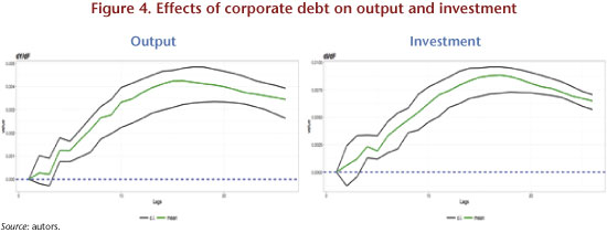
Excluding energy and food prices, so-called core inflation also shows signs of slowing down. In February 2023, it rose by 4.6% year-on-year, compared with 5.2% in September 2022. This dynamic can be explained in part by the evolution of durable goods prices, which were hit during 2022 by supply difficulties[4]. The indicator measuring the pressure on production lines has fallen sharply and, since the beginning of 2023, has returned below its long-term average value[5]. The impact of monetary policy will mainly be transmitted via demand. Indeed, the increase in the target rate for monetary policy has been passed on to all public and private rates, market rates and bank rates. The consequent tightening of monetary and financial conditions should result in a tapering of credit activity and a slowdown in domestic demand: consumption and investment.

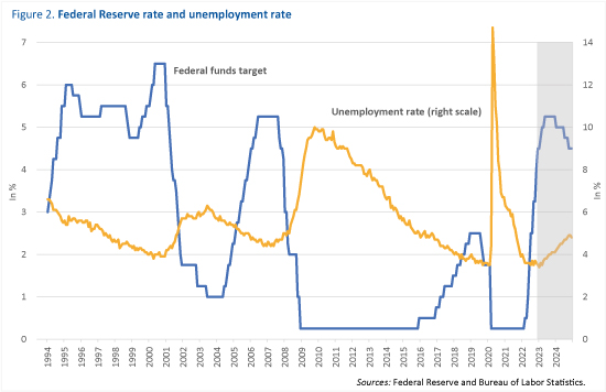
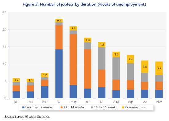
However, after GDP fell in two quarters at the beginning of 2022, it recovered in the second half of the year. Most importantly, the unemployment rate remains at a historically low level: 3.5%, according to the Bureau of Labor Statistics (BLS) for the month of March 2023. Is this situation – falling inflation without rising unemployment – sustainable? If so, the Federal Reserve would succeed in achieving its price target while avoiding recession or at least rising unemployment. Olivier Blanchard seemed to doubt this optimistic scenario. Indeed, most macroeconomic analyses suggest that a restrictive monetary policy pushes up unemployment. For example, the variant of the FRB-US model suggests that a one-point interest rate hike results in a 0.1 point rise in unemployment in the first year and then peaks at 0.2 points in the second and third years. Recent analysis by Miranda-Agrippino and Ricco (2021) suggests a similar order of magnitude, with a peak of around 0.2 points for a one-point increase in the policy rate, but faster transmission[6]. Given the magnitude of the monetary tightening and all else being equal, we expect the unemployment rate to rise by 0.3 percentage points in 2023, which in our scenario would bring it to 3.9% from 3.6% on average over 2022. Indeed, given the lags in the transmission of monetary policy, the tightening over 2022 is likely to have only a small impact, which could explain why the unemployment rate has not yet risen. Previous episodes of monetary tightening have also been characterised by a more or less significant lag between the tightening phase of monetary policy and an increase in unemployment (Figure 2). For example, the Federal Reserve’s moves to tighten monetary policy in the summer of 2004 did not have a rapid impact on the unemployment rate, which continued to fall until the spring of 2007, before rising sharply thereafter, reaching a peak of almost 10% in early 2010 in the context of the global financial crisis. The same inertia was evident after 2016, with unemployment not rising until 2020 during the lockdowns.

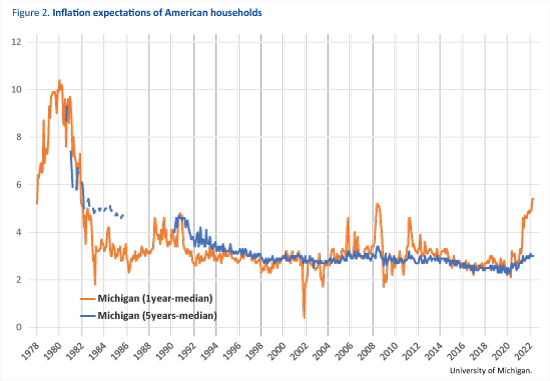
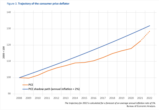
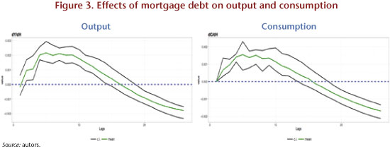
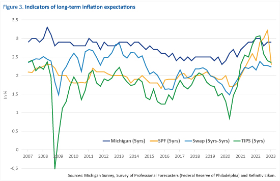
Finally, the capacity of monetary policy to reduce inflation depends not only on the relationship between unemployment and inflation but also on the reaction of inflation expectations. In this regard, the various indicators of long-term expectations suggest either stability or a slight decrease. For example, the Michigan Household Survey indicates a 5-year inflation expectation of 2.8% in February 2023, compared with 3.1% in June 2022. According to market indicators, 5-year 5-year forward inflation expectations fluctuate around 2.5%. These levels are certainly higher than the target set by the Federal Reserve, but they do not reflect a significant and lasting shift away from what was observed before 2021 (Figure 3). As for the inflation-unemployment link, it is clear that there is greater uncertainty. In the FRB-US model, the increase in unemployment induced by monetary tightening has very little effect on the inflation rate, although the estimates of Miranda-Agrippinon and Ricco (2021) suggest a greater impact. In our scenario, US inflation would continue to fall in 2023 not only because of the energy component but also because of a fall in core inflation. In our scenario, we assume that by the end of 2023, the deflator would rise by 3.6% year-on-year, with core inflation at 3.7%.

________________________________

[1] This is inflation measured by the consumer price deflator, which is the index monitored by the Federal Reserve. In comparison, inflation measured by the consumer price index (CPI) is on average higher, whether we consider the overall indicator or the index excluding food and energy prices.

[2] The price of gas on the US market has not reached the highs seen in Europe. However, the price almost tripled between the spring of 2021 and the end of summer 2022 before returning to the low point observed in April 2020.

[3] The contribution of food has already fallen since the start of the year, and we anticipate that this will continue.

[4] This is the case for semiconductors, used in particular by the automotive sector. These shortages have contributed to the rise in the prices of cars, both new and especially used, which rose by more than 40% year-on-year at the beginning of 2022.

[5] See the Global Supply Chain Pressure Index (GSCPI), which is calculated by economists at the New York Federal Reserve.

[6] See Miranda-Agrippino S. & Ricco G. (2021), “The transmission of monetary policy shocks”, American Economic Journal: Macroeconomics, 13(3), 74-107. Other estimates indicate effects that are sometimes greater, depending on the estimation strategy. See the simulations reported by Coibion O. (2012), “Are the effects of monetary policy shocks big or small?”, American Economic Journal: Macroeconomics, 4(2), 1-32.

by Christophe Blot

In the first quarter of 2022, US GDP fell by 0.4%, ending the recovery that had begun in the summer of 2020. The international economic environment had deteriorated significantly due to a combination of negative shocks. The global economic recovery has been accompanied by supply difficulties and a sharp upturn in energy prices, amplified since February 2022 by Russia’s invasion of Ukraine. The conflict has led to heightening geopolitical tensions and fuelled greater uncertainty[1]. Finally, rising inflation has led central banks, particularly the Federal Reserve, to raise interest rates. So is the decline in US GDP at the beginning of the year a sign of a recession, or will it simply put the brakes on growth?

After the steep downturn observed in 2020, the US economy rebounded sharply, and by the second quarter of 2021 GDP exceeded the level of activity seen at the end of 2019. Growth for 2021 as a whole stood at 5.7% and was strongly driven by domestic demand, in particular household consumption, which shot up by 7.9%[2]. The support plans implemented first by the Trump administration and then by Biden more than compensated for the loss of primary household income due to the pandemic, and generally boosted consumption, particularly of durable goods[3]. The dynamism of demand in the US and globally then ran up against supply constraints as new waves of COVID transmission struck. Although the spread of the virus in most countries was not accompanied by the kind of strict prophylactic measures taken in the spring of 2020, the situation nevertheless worsened, clogging up global supply chains and holding back labour supply[4]. This contrast between US demand, supported by highly expansionary fiscal policies, and constrained global supply has pushed prices up. In the US, the consumption deflator excluding energy and food prices rose to 3.3% in 2021, with much higher increases for some goods: 13.2% for cars, for example. Another sign of the imbalance in US growth: the sharp increase in import volumes (+14% over the year compared with a 4.5% increase in exports) has led to a deterioration in the trade balance in goods and services, with a deficit of $1,280 billion in 2021 (or 5.6% of GDP) compared with $905 billion (4.2% of GDP) two years earlier. The contraction of GDP observed in the first quarter of 2022 could be the manifestation of an overheating economy, as domestic demand has remained buoyant: +0.5 points. It is foreign trade’s negative contribution (-1 point) that accounts for the 0.4% fall in GDP. 

The rest of 2022 will be marked mainly by more negative shocks. While our October forecast anticipated growth of 4.2%, this figure had to be revised downwards significantly (Figure 1) to 2.1%. Although the US is an oil producer, the rise in price nevertheless is having a negative effect due to reduced household purchasing power and higher production costs for business[5]. Assuming that geopolitical tensions remain at the level observed in April until the end of the year, the uncertainty shock will cut growth by 0.4 points[6]. As for supply constraints, these should not have a major recessionary impact in the United States but will undoubtedly contribute to maintaining pressure on prices. The reduction in the growth forecast is also due in part to a stronger-than-expected tightening of monetary policy. Indeed, in the October 2021 scenario, we anticipated that inflation would gradually fall back to the Federal Reserve’s target, implying a much slower normalisation of monetary policy. In the face of the larger and longer-lasting inflationary shock, the Federal Reserve has tightened monetary policy. The last three meetings of the Federal Open Market Committee(FOMC) have resulted in consistent rate hikes, from 0.25% in January to 1.75% in June. This should continue in the second half of the year, with the rate increasing by 1.5 points on average over the year, which would have an effect on growth of up to 0.5 points from 2022. In total, these shocks should therefore cut the forecast for growth by 1.2 points. This effect is being compounded by the fact that actual growth in the third and fourth quarters of 2021 was less strong than we had anticipated: 0.6% and 1.7% respectively, compared with the October 2021 forecast of 1.4% and 2.3%. Finally, these shocks will not be offset by fiscal policy[7].

Given the figure for growth in the first quarter of 2022, quarterly growth during the following three quarters of around 0.3-0.4% should be compatible with annual growth of 2.1%[8]. The economic indicators for the months of April to June confirm a slowdown in US activity in a context of still high inflation. The monthly figures for household consumption, which rose in April (+0.3%) but fell in May (-0.4%), already suggest further slowing. This performance once again continues to be driven by purchases of durable goods, which peaked in March 2021 and have since fallen by 5.6% (Figure 2). Business confidence surveys have confirmed the slowdown, but levels are still above long-term averages. Moreover, industrial output continued to rise in April and May. Finally, on the employment and unemployment front, the figures for June provide a good picture of the second quarter. The unemployment rate stagnated at 3.6%, after having fallen by more than 11 points between April 2020 and March 2022. Employment in turn has risen on average from the first quarter, but the level in June 2022 was lower than in March. These elements therefore point to moderate or even negative growth, particularly if the contribution of foreign trade is again negative. At worst, however, this would be a technical recession[9].

[1] See “L’économie mondiale sous le(s) choc(s)” [The world economy in the face of shock(s)], OFCE Review, No. 177, for a detailed analysis.

[2] Total GFCF increased by 7.7%.

[3] See “Europe / États-Unis, comment les politiques budgétaires ont-elles soutenu les revenus?” [Europe / United States, how have fiscal policies supported incomes?], OFCE the Blog, 26 October 2020.

[4] China was a notable exception because of its “zero Covid” strategy, resulting in local lockdowns.

[5] A recent review of the literature does suggest that higher oil prices reduce household consumption and investment. See A. M. Herrera, M. B. Karaki & S. K. Rangaraju, 2019, “Oil price shocks and US economic activity”, Energy policy, No. 129, pp. 89-99.

[6] See Table 3 on page 32 of “L’économie mondiale sous le(s) choc(s)“, Op. cit.

[7] The estimate of the impact of fiscal policy reflects the revision of the fiscal impulse compared to the scenario envisaged in October 2021. The fiscal impulse was negative due to the end of various one-off measures enacted to address the health crisis. The revision is mainly due to the analysis of the measures included in the 2022 budget by the Biden administration.

[8] The performance in Q1 may well already partly capture the impact of the various shocks.

[9] A technical recession refers to a situation when GDP declines over two consecutive quarters. However, a recession depends on a set of indicators.

by Christophe Blot

At the monetary policy meeting on 16 March 2022, the Federal Reserve raised its interest rate by a quarter point to 0.5%[1]. With the strong increase in inflation observed in the United States since the spring of 2021, there is little doubt that this movement will continue. Indeed, Jerome Powel recently confirmed this and envisaged a half point increase at the meeting on 4 May. Beyond that, expectations from futures contracts on the federal funds rate suggest that the interest rate will rise to at least 3% by year’s end. Will the US central bank succeed in bringing inflation back to its target? Put another way, can the nature of the imbalances that are pushing up prices be corrected by monetary policy? And how high should interest rates rise to curb the current inflationary surge?

After settling at 1.2% in 2020, inflation, measured by the consumer price deflator, reached 3.9% in 2021 on an annual average, i.e. a level well above the Federal Reserve’s 2% target[2]. Furthermore, contrary to the expectations formulated by the members of the Federal Open Market Committee (FOMC) in mid-2021,[3] inflation picked up steam and by February 2022 exceeded 6%, the highest level since 1982[4]. As Jean-Luc Gaffard and Francesco Saraceno point out, inflation is necessarily the result of sectoral market imbalances, which have their source in either insufficient supply or excess demand. The appropriate policy response must therefore be based on as complete a diagnosis as possible of the causes of the inflation, which results in social costs[5]. However, given the Fed’s mandate, tightening monetary policy seems unavoidable[6]. In the case of the United States, this is a dual mandate since, according to the Federal Reserve Act, the aim of US central bank policy is to promote both price stability and maximum employment. With the unemployment rate at 3.6% in March 2022, the Fed logically considers that it is further from its price stability objective than from its full employment objective. Besides the unemployment rate, other indicators such as the resignation rate or the ratio between the number of unemployed and job openings also confirm the existence of tensions on the labour market[7].

The main question is therefore how much tightening is needed to bring inflation back to target. The answer to this question depends in particular on the transmission of monetary policy to prices. How does inflation react when the central bank decides to raise its interest rate? Remember that the central bank only sets a very particular rate, a very short-term money market rate. Changes in this rate are then transmitted to market and bank rates, and on to financial and property prices. Monetary policy therefore influences the totality of financing conditions and, through this, household consumption and household and business investment[8]. When the central bank tightens its monetary policy, demand is reduced and unemployment rises, which has an impact on prices, i.e. the prices of goods and services and wages. The impact of monetary policy on inflation can be quantified by estimating the effect of higher interest rates on unemployment and the link between inflation and unemployment.

A recent analysis by Silvia Miranda-Agrippino and Giovanni Ricco (2021) suggests that a one percentage point hike in the interest rate set by the central bank pushes up the unemployment rate by 0.3 percentage points after 12 months.[9] All else being equal, Ball and Mazumder (2011) suggest that, using a standard Phillips curve estimate, an additional 1 percentage point of unemployment would reduce inflation by 0.5 percentage points. So raising the rate from 0.25% to 3% by the end of 2022 would result in a 0.4 percentage point reduction in inflation. The tightening scenario envisaged for monetary policy therefore seems largely insufficient to bring inflation back to its 2% target. In other words, the only way the Fed could hope to reduce inflation would be by raising the interest rate even further. This is not, however, a reasonable prospect.

First, reducing inflation by 4 points – from 6% to 2% – implies such a steep rate hike that it would push the US economy into a violent recession and a brutal rise in unemployment. This was the path chosen by Paul Volcker, Fed Chairman between 1979 and 1987, who pursued a highly restrictive monetary policy at the beginning of his term in order to reduce US inflation, which exceeded 10% at the end of 1979 (Figure 1). The result was a sharp rise in the unemployment rate, to its highest level since 1951[11]. There are, however, important differences with the current inflationary situation. Inflation today is partly the result of supply factors that, according to Reifschneider and Wilcox (2022), are temporary[12]. Monetary policy would not be effective in countering a shock to energy prices or global supply constraints, since these do not really depend much on the US macroeconomic situation. The point is to focus action on the contribution to inflation arising from domestic factors, and in particular tensions on the labour market, which have been fuelled in part by the fiscal stimuli of Donald Trump in 2020 and then of Joe Biden in 2021[13]. However, it is clear that, like many other forecasters, the Fed was off in its belief that this inflationary episode would not last long and that supply factors would ease relatively quickly. Since then the war in Ukraine has put further pressure on energy prices and hence on inflation.

At the same time, it seems apparent that inflation expectations are probably better anchored around the Federal Reserve’s inflation target than they were in the late 1970s. According to the Michigan Household Survey, long-term inflation expectations – five years ahead – have risen but appear to have stabilised around 3% since May 2021. In particular, they are lower than they were in the late 1970s and early 1980s (Figure 2). And these inflation expectations do play a role in the dynamics of inflation. Indeed, the more households or companies anticipate a high level of inflation, the more they will ask for wage increases or set their prices at a higher level, which will result in a spiral in which inflation expectations feed inflation, which in turn pushes expectations a little higher. It is therefore also in order to avoid this type of runaway so-called second-round effects that the Fed is deciding to accelerate its monetary tightening. The aim is to maintain this anchorage. Recent work has shown that this channel for transmitting monetary policy onto expectations is significant[14].

It therefore seems that the current situation justifies monetary tightening in the US. The difficulty facing the central bank is to distinguish between supply and demand factors. The objective of the tightening initiated by the Fed must be mainly to limit the tensions observed on the labour market and to influence agents’ expectations so that these expectations don’t take off. It should at the same time be relatively moderate so as not only to avoid pushing the economy into recession but also to avoid a sharp rise in long-term interest rates, which would lead to destabilising pressures from the weight of the public debt. While the supply factors driving inflation are temporary, the Fed’s response will allow inflation to gradually converge towards its target. In this respect, it is worth noting that the average inflation targeting strategy gives the Fed greater manoeuvring room, as it can in fact tolerate inflation above 2%. Since 2008, inflation has mostly been below 2%, so even with 5% inflation in 2022, the path of the price index would still be lower than the shadow path that would have been observed if inflation had risen by 2% per year since 2009 (Figure 3). Finally, if the supply factors prove to be long-term, the appropriate economic policy will not be to curb demand through an overly restrictive economic policy but rather to stimulate supply through an investment policy that can raise production capacity to the appropriate level.

[1] In the United States, the Federal Reserve’s policy rate corresponds to the target for the rate at which commercial banks exchange federal funds, which are the deposits they hold with the local Federal Reserve.

[2] See Blot, Bozou and Hubert (2021) for a discussion of central bank inflation targets and the reformulation proposed by the Fed in August 2020.

[3] Projections by FOMC members in June 2021 suggested inflation of between 1.9% and 2.3% at the end of 2022, with a median of 2.1%: see here.

[4] Inflation measured by the consumer price index even exceeded 8.5% in March 2022. Note that the inflation indicator used by the Federal Reserve is the consumer price deflator.

[5] Even if wages are growing faster in the US, they are not currently compensating for inflation, which is resulting in a loss of purchasing power for US households.

[6] Basically, the central bank’s mandate does not specify that its monetary policy response should be differentiated according to the causes of inflation, which implicitly suggests that long-term inflation can only be a monetary phenomenon.

[7] See this analysis or this one.

[8] Monetary policy also influences foreign trade through its effect on the exchange rate.

[9] See Miranda-Agrippino S., & Ricco G. (2021). The transmission of monetary policy shocks. American Economic Journal: Macroeconomics, 13(3), 74-107. The effect on unemployment is obtained by considering a monetary policy shock such that the one-year interest rate rises by one percentage point. Although the Federal Reserve does not directly control this rate, it is nevertheless influenced by the central bank’s decisions.

[10] See Ball L. M. & Mazumder S. (2011). Inflation dynamics and the great recession. Brookings Papers on Economic Activity, Spring, 337-381.

[11] This record of 10.8% in November 1982 was only exceeded in April-May 2020 during the pandemic. In 2009, the peak for the unemployment rate rose to 10%.

[12] See https://www.piie.com/sites/default/files/documents/pb22-3.pdf. Their optimism is, however, debatable.

here: https://www.piie.com/blogs/realtime-economic-issues-watch/what-needed-tame-us-inflation

[13] See Aurissergues, Blot and Bozou (2021), “Les États-Unis vers la surchauffe? [Is the US overheating?] Policy Brief of the OFCE no. 97

[14] See Diegel M. & Nautz D. (2021), “Long-term inflation expectations and the transmission of monetary policy shocks: Evidence from a SVAR analysis”, Journal of Economic Dynamics and Control, 130, 104192.

by Elliot Aurissergues, Christophe Blot and Caroline Bozou

The latest inflation figures for the United States
confirm the trends seen over the last few months. In October 2021, consumer
prices rose by 6.2% year-on-year. While rising prices is a global phenomenon, among
the industrialized countries this has been particularly marked in the US. Inflation
in the euro zone over the same period was 4.1%. This level of increase in
inflation has not been seen since the late 1990s, so it is attracting
considerable attention in the US policy debate, not least because it echoes a
controversy that began early in Joe Biden’s mandate over the fiscal stimulus
passed in March 2021. Although inflation is being driven in part by rising energy
prices, the fact remains that tensions have rapidly increased. Excluding energy
and food components, inflation has exceeded 4% since June 2021, suggesting a
risk of overheating for the US economy. While the European macroeconomic
context does not allow us to identify an equivalent risk for the euro zone, the
fact remains that a sustained rise in US inflation could have repercussions for
the zone. Beyond the impact on competitiveness, the dynamics of US inflation
could influence decisions on rate changes and the conduct of monetary policy by
the Federal Reserve and the European Central Bank.

Regardless of the indicator – consumer price index
or consumption deflator – prices have clearly accelerated since March 2021 (see the figure)[1]. The energy component is undoubtedly important,
but it does not fully explain this dynamic, since the latest figures for the
underlying indices, i.e. adjusted for energy and food prices, show a
year-on-year increase of 4.6% for the CPI and 3.6% for the consumption deflator[2]. Note too that this development reflects a
catch-up from 2020, when inflation was particularly moderate in the context of
the pandemic and the sudden halt in activity. Thus, on average over 2020 and
2021, up to October, the consumption deflator has risen by 2.1%, in line with
the target adopted by the Federal Reserve[3]. The recent tensions obviously reflect the
dynamics of the post-lockdown global economic recovery, which the United States
is clearly part of, and which has led to strong pressure on energy prices, but
also on supplies, as evidenced by the supply difficulties for certain goods and
the soaring cost of maritime freight.

Beyond these global factors, there is the question
of an inflationary phenomenon that may be intrinsically linked to US economic
policy. Even before the recent discussions on the 2022 budget vote, the
measures taken to deal with the Covid crisis first by the Trump administration
and then by the Biden administration amount to a grand total of USD 5.2
trillion, representing more than 23 points of GDP for the year 2019. This
spending over 2020 and 2021 represents an unprecedented level of stimulus over the
last forty years. While there was undoubtedly a consensus on the need for the
measures proposed by Biden and approved by Congress in March 2021, their
magnitude nevertheless caused a great deal of debate, as the recovery was
already underway and the economy was already benefiting, as it still is today,
from the fiscal support measures voted in 2020 and from a highly expansionary
monetary policy[4]. Could this expansionary economic policy – both fiscal
and monetary – be causing the economy to overheat, fuelling the return of
inflation, as economists such as Lawrence Summers and Olivier Blanchard fear,
or, on the contrary, is the effect on inflation being overestimated, as other
analyses suggest? We plunge into this debate in an OFCE
Policy Brief,
specifying in particular the conditions that could lead to a sustainable
increase in inflation. The risk will depend on the size of the multipliers
measuring the effect of the stimulus plans on activity and unemployment, the
position of the US economy relative to its potential, and changes in inflation
expectations, all of which are subject to some uncertainty.

[1] The consumer price index (CPI) is calculated from
a survey of the prices of a basket of average goods consumed by a
representative household. The consumption deflator is derived from the national
accounts and represents the price system that allows the transition from
consumption in value to consumption in volume. See La désinflation importée [Imported
Deflation] in OFCE Review, 2019, No. 162, for more details on the
difference between these two measures of inflation.          

[2] Unadjusted for energy and food prices, the
consumption deflator rose by 4.4%. The data for the deflator refer to the month
of September, while the publication of the consumer price indices is more
rapid, the latest figures published being those for October.

[3] The consumer price deflator is the indicator used
by the Federal Reserve to assess price stability in the United States.

[4] Two other projects were then announced: an
infrastructure investment plan (American Jobs Plan)
and a household package (American Families Plan).
These are not crisis-specific measures, but measures that are supposed to mark
the direction of fiscal policy over the next eight years. These plans are
currently being discussed in Congress as part of the 2022 budget vote.

By Christophe Blot

As with the economic performance of all the industrialized
countries, economic activity fell off sharply in the second quarter of 2020
across the Atlantic before rebounding just as sharply the following quarter. The
management of the crisis in the US is largely in the hands of the different States,
and the election of Joe Biden should not change this framework since he
declared on November 19 that he would not order a national lockdown. However,
the health situation is continuing to deteriorate, with more than 200,000 new Covid-19
cases per day on average since the beginning of December. As a result, many
States are adopting more restrictive prophylactic measures, although without returning
to a lockdown like the one in the Spring. This situation could dampen economic prospects
for the end of the year and also for the start of the mandate of the new
President elected in November. Above all, it makes it even more necessary to
implement a new recovery plan, which was delayed by the election.

As in the euro zone, recovery in the US kicked off as
soon as the lockdown was lifted. GDP grew by 7.4% in the third quarter after
falling by 9% in the previous quarter. Compared with the level of activity at
the end of 2019, the economic downturn amounted to 3.5 points, versus 4.4
points in the euro zone. The labour market situation also improved rapidly,
with the unemployment rate falling by 8 points, according to data from the Bureau
of Labor Statistics for November, from its April peak of 14.7%. These results
are the logical consequence of the lifting of restrictions but also of the large-scale
stimulus plans approved in March and April, which have massively absorbed the
loss of income for households and to a lesser extent for US companies (see here).
However, the upturn in consumption is still being dampened by some ongoing restrictions,
particularly in sectors with strong social interactions, where spending is
still nearly 25% lower than it was in the fourth quarter of 2019 (Figure 1).
As for the consumption of goods, it has been much less
affected by the crisis and is down only 12% from its pre-crisis level for
durable goods and 4.4% for non-durable goods. Nevertheless, most of these
support measures have come to an end, and as of this writing the discussions
that began in late summer in Congress have not yet led to an agreement between
Republicans and Democrats. Despite the rebound, the health impact of the pandemic
and the economic consequences of the lockdown on the labour market require a discretionary
policy in a country where the automatic stabilizers are generally considered to
be weaker[1]. New support measures will be all the more
necessary as a further tightening of restrictions is looming and the recovery
seem to be running out of steam. The initial consumption figures for the month
of October point to a fall in the consumption of services, and employment also
stabilized in November, remaining well below its level at the end of 2019.

However, after the setback of the discussions in
Congress, it will now be necessary to wait until the first quarter of 2021 for
a new support plan to be approved and for a possible reorientation of US fiscal
policy after Joe Biden’s victory. In the Autumn, the Democrats proposed a 2
trillion dollar (9.5 GDP points) package, almost as much as the 2.4 trillion dollar
(10.6 GDP points) package adopted in March-April 2020[2]. The aid would, among other things, support the
purchasing power of the unemployed through an additional federal payment.
Although unemployment is much lower than in the second quarter, it remains
above its pre-crisis level and is now characterized by an increase in long-term
unemployment for which there is generally no compensation. In November, the
share of those who had been unemployed for at least 27 weeks was 37 per cent
(or 3.9 million people, Figure 2), and the median duration of unemployment
had risen from 9 weeks at the end of 2019 to almost 19 weeks in November 2020.
In addition, States whose tax revenues have decreased with the crisis could
benefit from a federal transfer, thereby avoiding spending cuts[3].

However, despite the end of the suspense over the
outcome of the presidential elections, the political and economic uncertainty
has not been completely resolved. Indeed, it will not be known until early
January whether the Democrats will also have a majority in Congress. They have
certainly kept the House of Representatives, but it will be necessary to wait
until the beginning of January for the Senate, with a ballot planned in Georgia
that will determine the political colour of the last two seats [4]. Both seats are now held by Republican senators.
However, Joe Biden won Georgia by 0.2 points against Donald Trump, the first
victory in the State for a Democratic candidate since 1992. With both State-wide
senatorial elections to be contested directly, the results are likely to be
close.  If one of the Democratic
candidates is defeated, Joe Biden will be forced to contend with the
opposition. But, as Paul Krugman
points out, the Republicans are generally more inclined, once in opposition, to
promote austerity. This is reflected in the uncertainty indicators of Bloom,
Baker and Davies, whose economic policy uncertainty rose in November (Figure 3).
This uncertainty is certainly lower than in the Spring but remains higher than
that observed between 2016 and 2019. During this period, growth could weaken,
and then a strong recovery is likely to be followed by more subdued growth,
which will have repercussions on the labour market. Regardless of the outcome,
a plan will likely be approved in the first quarter of 2021, but its adoption
could take longer if it is conditional on an agreement between Republicans and
Democrats in Congress. However, this could be lengthy given the urgency of the
health and social crisis, and could plunge a significant proportion of the most
vulnerable into poverty.

Source : Baker, Bloom & Davis. https://www.policyuncertainty.com/index.html

[1] See for example Dolls, M., Fuest, C. &
Peichl, A., 2012, “Automatic stabilizers and economic crisis: US vs. Europe”, Journal of Public Economics,
96(3-4), pp. 279-294.

[2] By comparison, the
European programmes are weaker, ranging from 2.6 GDP points for France to 7.2
points for the UK.

[3] Note that the States generally have fiscal
rules limiting their capacity to run a deficit.

[4] Of the 100 seats in the Senate, the
Republicans already hold 50. In the event of a tie between the two parties, it
is the voice of the Vice-President-elect Kamala Harris that will decide between
them. A single victory in Georgia would therefore allow the Republicans to
retain the majority.

By Christophe Blot, Magali Dauvin and Raul Sampognaro

The sharp fall in activity and its brutal social consequences have led governments and central banks to enact ambitious support measures to cushion the shock, which resulted in an unprecedented global recession in the first half of 2020, as discussed in Policy Brief 78 . Faced with a health crisis that is unprecedented in contemporary history, requiring forced shutdowns to curb the spread of the virus, governments have taken urgent measures to prevent the onset of an uncontrolled crisis that could permanently alter the economic trajectory. Three main types of measures have been taken: some aim to maintain consumer purchasing power in the face of the shutdowns; others seek to preserve the production system by targeting business; and some are specific to the health sector. The quarterly national accounts, available at the end of the first half of the year, provide an update on the extent to which the disposable income of private agents has been preserved by fiscal policy at this stage of the Covid-19 crisis [2].

Fiscal policy has shot up Americans’ household
income and preserved Europeans’ income

In the major advanced economies, the Covid-19
crisis generated losses in primary income (before cash transfers) ranging from 81
billion pounds in the United Kingdom to 458 billion dollars in the United
States (Table 1). The initial income shock was thus larger in Spain and Italy –
6.5 and 6.7 GDP points respectively – and smaller in Germany (3.4 GDP points)
and the United States (2.1 GDP points).

Figure 1 breaks down the share of the primary income (PI) shock received by agents (first bar on the left for each country, labelled “PI”). In Spain and Italy, households suffered the majority of the losses, accounting for 54 percent and 60 percent, respectively, of the total income loss for the economy. In France and Germany, enterprises bore the lion’s share  of the income loss (48%). In the United Kingdom and the United States, enterprises incurred losses of £50 billion and $275 billion, respectively, accounting for 62% and 60% of the total loss for the economy. General government (GG) experienced a smaller shock in all the countries, which is explained by the spontaneous changes in some of the automatic stabilizers, and by a relatively lower value added due to the restrictions on activity during lockdowns.

Turning to the breakdown in losses in disposable
income (DI), which takes into account cash transfers, social contributions, and
income tax, the story is rather different. The implementation of emergency
measures made it possible to absorb some of these losses, as illustrated by the
bar labelled “DI” in Figure 1. The introduction of short-time working
in European countries thus shifted the burden of wages from enterprises to the
government, thus preserving household incomes and avoiding the termination of job
contracts. Similarly, reductions in social contributions and tax on income and
corporate profits have shifted the cost of the crisis from private agents to
government. In the face of the unforeseeable shock, the State has thus played
the role of insurer of last resort of private agent income, although to
different extents in different countries. Thus, while Spain’s government absorbed
13.5 percent of the primary income shock, support measures raised this share to
59 percent, a higher level than that of Italy (55.3 percent) and France (54.3
percent) in terms of disposable income. In comparison, the measures taken by
the German government absorbed a higher share of the shock, amounting to 67
percent of the loss of disposable income, compared with 28 percent of the fall in
primary income.

In the United Kingdom, emergency measures absorbed
the entirety of the shock. While business and households suffered primary
income losses of £50 billion and £15 billion respectively, their disposable
income fell by only £4 billion and £2 billion. As for disposable income,
government absorbed 93.6 percent of the shock. The contrast is even more marked
in Germany and the United States, where measures overcompensated the initial
primary income shock, especially for households. The US figures are
particularly impressive. Over the six-month period, primary income fell by $192
billion, while household disposable income rose by $576 billion, due in
particular to the payment of a tax credit and an exceptional federal
unemployment benefit of $600 per week that was paid to the unemployed,
regardless of their initial income[3]. The various tax measures and subsidies to
business reduced the loss by $210 billion. The US government thus absorbed 237
per cent of the shock, reflecting the magnitude of the support measures taken
in March-April.

Job losses and uncertainty about the future may
hamper recovery across the Atlantic

As we have seen, fiscal policy has been mobilized
massively across the Atlantic. Even if at this stage the macroeconomic shock has
been weaker in the US than in the EU[4], the fiscal impulse is much larger. At the end of
the first half-year, total transfers to households exceeded the immediate shock
to their primary income. This has led to a 13% increase in the disposable
income of US households, at the same time as their primary income fell by 4% in
connection with job destruction. This situation is due in particular to a tax credit
paid to households and an additional lump-sum allowance of $600 per week paid
by the federal government to any person eligible for unemployment. Between Q4 of
2019 and Q2 of 2020, transfers to households leapt by 80%, now representing 31%
of disposable income compared with 19% in 2019.

This difference in crisis management is undoubtedly
explained by the weakness of the social safety net in the United States, which
effectively reduces the role of automatic stabilizers while also limiting the
ability of citizens with little or no health insurance coverage to meet health
care expenses in the event of a fall in income. The use of counter-cyclical
measures is thus of greater importance, which probably explains why the
stimulus packages are more extensive than they were during the 2008-2009 crisis
as well as why the measures provide direct, substantial support to household
income. Moreover, in the US, the federal government is responsible for this
stimulus, while in the EU, the bulk of the support plans come from the Member states.

The sharp rise in unemployment across the Atlantic
– which peaked at 14.7% in April – contrasts with the situation in Europe,
partly due to the differentiated strategy in economic policy. The United States carried out a positive, substantial
transfer of income to households to offset the fall in wages resulting from job
losses, which also helped to mitigate the shock on business margins.
Conversely, in the main European economies, contractual employment
relationships were maintained, but household incomes were not preserved quite
as much – they actually fell slightly, except in Germany. In the main European
economies, a decision was taken to use short-time working on a massive scale, while
in the United States the response was to send cheques directly and immediately
to households.

This situation, where income was propped up during
a period when consumption was curtailed by the closure of non-essential shops, led
to the accumulation of 76 billion euros in “Covid savings” in Germany
(8 GDI points), 62 billion in France (9 GDI points) and 38 billion in Spain and
Italy (10 and 6 GDI points respectively). In the United Kingdom and the United
States, “Covid savings” were even greater: £89 billion in the UK (12 GDI
points), while the sum reached $961 billion in the US (12 GDI points). How the
epidemic develops and how these savings are used will be the two keys
determining the extent of the rebound in activity starting in the second half
of 2020.

This is precisely the moment when differences in
approach can create divergences in economic trajectories. While it could be
said that up to now household situations have been better preserved across the
Atlantic, job contracts have been shredded. In this context, it may take some
time to get the workforce back into employment, hindering the rapid
redeployment of the production base. This could slow down the speed at which activity
returns to normal, helping to keep job losses up and limiting the restoration
of company balance sheets. Furthermore, negotiations between Democrats and
Republicans in Congress have hit the wall of the approaching November 3
elections. If the measures taken during the crisis are not – at least partially
– renewed, the situation of American households is likely to become more
critical, since weak US social safety nets will not be able to mitigate what
threatens to be a long-term shock. This may have second-round effects on
primary income and investment [5]. Following the elections, further measures are
likely to be taken, but the time lag could be long, especially if Joe Biden
wins, as he will have to wait until he takes office in January 2021. Continued
high uncertainty about the extent of the recovery – accentuated by political
uncertainty – may encourage American households to avoid spending “Covid
savings” in order to have “precautionary savings” to face a probable
long-term health, economic and social crisis.

Glossary

Primary income (PI): Primary income includes revenue directly related
to participation in the production process. The bulk of primary household
income consists of wages, salaries and property income.

Gross disposable income (GDI): Income available to agents to consume or invest,
after redistribution operations. This includes primary income plus social cash
benefits and minus social contributions and taxes paid.

* * *

[1] See “Evaluation de la pandémie de Covid-19 sur
l’économie mondiale” [Evaluation
of the Covid-19 pandemic on the world economy], Revue de l’OFCE no. 166 for
an initial analysis of the various fiscal and monetary support measures
implemented.

[2] These results should be taken with a grain of
salt. While the quarterly national accounts are the most comprehensive,
consistent framework available, with data collected by official statistics
institutes, they are nevertheless provisional. These accounts are subject to
significant revisions that may significantly alter the final results when they
incorporate new data (company balance sheets, etc.); they are considered final
within two years.

[3] This allowance is in addition to that paid by
State-run unemployment insurance systems.

[4] The loss in 6-month GDP was 5% in the US,
compared with 8.3% in the EU.

[5] F. Buera, R. Fattal-Jaef, H. Hopenhayn, A.
Neumeyer, and J. Shin (2020), “The Economic Ripple Effects of COVID-19”, Working Paper.

By Christophe
Blot

In the United States as in France, the
COVID-19 crisis has led to numerous measures restricting economic activities intended
to limit the spread of the virus. The result will be a fall in GDP, which is already
showing up in figures for the first quarter of 2020, and which will be much steeper
in the second quarter. In a country noted for its weak employment protection,
this unprecedented recession is quickly having repercussions on the labour
market, as reflected in the rise in the unemployment rate from a low point of 3.5%
in February to 14.7% in April, a level not seen since 1948. As Bruno
Ducoudré and Pierre Madec have recently demonstrated in the case of France,
the current crisis in the United States should also result in heightened inequalities
and insecurity. And the shock will be all the greater in the US since the
social safety net is less extensive there.

In the United States, the Covid-19 restrictions
were set not at the Federal level but by the various States at differing times.
The vast majority of States did decide however to close schools and
non-essential businesses and to encourage people to stay home. The lockdown was
thus imposed by California on March 19, followed by Illinois on March 21 and
New York State on March 22, but South Carolina didn’t follow until April 6.
North Dakota, South Dakota, Arkansas, Iowa and Nebraska have taken no action,
and three other States – Oklahoma, Utah and Wyoming – applied measures only in certain
counties, and not State-wide. However, by early April a large part of the
country had been locked down, with a varying degree of strictness, affecting between
92% and 97% of the population[1].

Which employees have been hit hardest by the crisis?

According to a survey by the US Bureau of Labor Statistics, almost 25%
of employees worked from home in 2017-2018. However, some employees said they
could have stayed at home to work but did not necessarily do so during the
reporting period. With the COVID-19 crisis and the incentives to modify the
organization of work, we can therefore consider that almost 29% of employees
could stay at home during the lockdown [2].
Furthermore, as the survey
carried out for France highlights, the implementation of teleworking is more
widespread among employees in management jobs and commercial or financial
activities. In 2017-2018, 60% of these people could have managed to work from home.
In contrast, fewer than 10% of workers in agriculture, construction, manufacturing
or transport services would have been able to telework during the crisis. Not surprisingly,
the survey also shows that the employees able to telework are also those at the
top of the wage distribution. For the top quartile, 61.5% of employees could
work at home compared with fewer than 10% for employees in the bottom quartile.

Mirroring these
elements, a more recent study analyzed which jobs would be most affected by the
lockdowns and in particular by the closure of non-essential businesses [3]. Six sectors are particularly exposed.
Logically enough, these include bars and restaurants, transport and travel,
entertainment, personal services, the retail trade and some manufacturing
industries. Based on employment data for the year 2019, these sectors represent
20.4% of total employment. With more than 12 million jobs, the bar and
restaurant sector is being hit hardest. This survey also shows that the most
exposed employees generally receive below-average pay. They are particularly
concentrated in the two lowest wage deciles. For example, the wage bill for bar
and restaurant workers represents barely 3% of the total wage bill but more
than 8% of employment. These people usually work in companies with fewer than
10 employees. This dimension is all the greater in the United States since
access to health insurance is often linked to the employer, whose obligations for
insurance provision depend on how many employees they have. Finally, by
crossing the distribution by sector and geography, it appears that Nevada,
Hawaii and to a lesser extent Florida (23.7%) concentrate a larger share of these
sectors, and therefore of the exposed jobs [4]. Conversely, Nebraska, Iowa and Arkansas
are among the States where these sectors account for a smaller share of
employment [5]. These three States have also not adopted lockdown
measures and should therefore be relatively spared from the rise in unemployment.

Unemployment statistics for the months of
March and April
confirm this outlook. In one year, the unemployment rate increased by 4.8
points for those in management jobs or commercial or financial activities,
while, over the same period, the rate rose by 23 points for service jobs and
almost 15 points for employees in production. The geographic disparities are
also significant. In California and Illinois, the first States to implement a
lockdown, the unemployment rate rose 11.3 and 12.2 points, respectively, in one
year. Conversely, the States that have not enacted lockdown measures are among
those where the unemployment rate has risen the least over the year. The
increase reached 5.2 points for Nebraska, 6.7 points for Arkansas and 7.5
points for Iowa, for example.

The structure of employment is, however, a
key factor determining the variation in unemployment. Despite fairly close starting
dates for the lockdowns in Connecticut and Michigan, the unemployment rate rose
only 4.2 points in the former versus over 18 points in industrial Michigan. The
statistics also confirm the exposure to the shock of Nevada and Hawaii, which
recorded the two largest increases: 24.2 and 19.6 points respectively, while
Minnesota, with a very low exposure, saw its unemployment rate rise by only 4.9
points, one of the smallest variations since April 2019. Likewise, the impact
has been relatively softer in the District of Columbia, where the unemployment
rate rose by 5.5 points.

Health under threat?

The deteriorating state of the labour
market will be accompanied by a deterioration in living conditions for millions
of Americans, especially if the end of the lockdowns is not synonymous with a
rapid rebound in activity, as Jerome Powell, Chairman of the Federal Reserve,
now fears. This would result in increased poverty for households that have lost
their jobs. Previous analyses indicate that workers at the bottom of the
distribution will be the most exposed, especially since, despite the measures taken to
extend unemployment insurance, the duration of benefits remains overall
shorter in the United States. To deal with the crisis, the Federal government
has spent USD 268 billion (or 1.3 percentage points of GDP) on unemployment
insurance to extend the duration and amount of compensation. This is in
addition to the tax credit of up to USD 1,200 for households without children [6].
The government has thus chosen to support incomes temporarily, but unlike the
partial unemployment schemes in force in France and in many other European
countries, it has not protected jobs [7].
The flexibility of the US labour market could, however, prove more advantageous
in so far as the recovery is rapid and differs depending on the sector.
Employees actually do not lose much of their skills and can more easily find a
job in another business sector. But a protracted crisis associated with persistently
higher unemployment would greatly increase poverty.

In addition, access to health insurance is
also often linked to employment. Indeed, 66% of insured Americans are covered
by their employer, who is obliged to offer health insurance in companies with
more than 50 employees. The corollary is that many workers risk losing their
health coverage at the same time as their jobs if they cannot pay the portion of
the insurance costs previously borne by their employer. As for employees of
small businesses exposed to the risk of closure and unemployment, it is very
likely that they will no longer have the means to take out a private insurance
policy on their own. Already, in early 2019, just over 9% of the population had
no health coverage. While this rate had dropped sharply since 2010 and the
“Obamacare” reform, the annual report
of the US Census Bureau published in November 2019 estimated that more than 29
million people had no coverage in 2019, a figure that has risen somewhat since
2017. The coverage rates also show strong regional disparities, which is due to
the demographic structure of the States.

Although part of the economic support plan
is devoted to food aid [8]
and some health expenses, the COVID-19 crisis will once again hit the most
vulnerable populations and widen inequalities that are already significant and being
deepened by the recent tax reforms of the Trump administration.

[1]
In terms of GDP, the share of States that have imposed lockdowns is in much the
same proportions.

[2]
Note that this survey does not show a significant difference between men and
women, even if women have a slightly fewer opportunities for teleworking: 28.4%
against 29.2% for men.

[3]
See Matthew Dey and Mark A. Loewenstein, “How
many workers are employed in sectors directly affected by COVID-19 shutdowns,
where do they work, and how much do they earn?”, Monthly Labor Review,
U.S. Bureau of Labor Statistics, April 2020.

[4]
In Nevada, the exposed sectors represent 34.3% of jobs. This figure also
exceeds 30% in Hawaiï and is 23.7 % in Florida.

[5]
This is also the case of the District of Columbia due to the large presence of Federal
employees.

[6]
This amount is granted to households
receiving less than USD 75,000 (150,000 for a couple) per year. USD 500 is
awarded per child. The amount of the tax credit is regressive and falls to zero
for households with an income above USD 99,000.

[7]
See here
for our analysis of European and American strategies to deal with the crisis.

[8]
The plan approved on 18 March (Families
First Coronavirus Response Act) actually provides for over 20 billion
dollars in assistance for poor people.

By Christophe Blot

While the momentum for growth has lost steam in some countries – Germany, France and Japan in particular – GDP in the United States is continuing to rise at a steady pace. Growth could even pick up pace in the course of the year as a highly expansionary fiscal policy is implemented. In 2018 and 2019, the fiscal stimulus approved by the Trump administration – in December 2017 for the revenue component, and in February 2018 for the expenditure side – would amount to 2.9 GDP points. This level of fiscal impulse would come close to that implemented by Obama for 2008. However, Trump’s choice has been made in a very different context, since the unemployment rate in the United States fell back below the 4% mark in April 2018, whereas it was accelerating 10 years ago, peaking at 9.9% in 2009. The US economy should benefit from the stimulus, but at the cost of accumulating additional debt.

Donald Trump had made fiscal shock one of the central elements of his presidential campaign. Work was begun in this direction at the beginning of his mandate, and came to fruition in December 2017 with the passing of a major tax reform, the Tax Cuts and Jobs Act [1], which provided for a reduction in household income tax – in particular by reducing the maximum marginal income tax rate – and corporation tax, whose effective rate would fall from 21% to 9% by 2018 [2]. In addition to this initial stimulus, expenditure will also rise in accordance with the agreement reached with the Democrats in February 2018, which should lead to raising federal spending by USD 320 billion (1.7 GDP points) over two years. These choices will push up domestic demand through boosting household disposable income and corporate profitability, which should stimulate consumption and investment. The multiplier effect – which measures the impact on GDP of a one dollar increase in public spending or a one dollar cut in taxes – will nevertheless be relatively small (0.5) because of the US position in the cycle.

Moreover, the public deficit will expand sharply, to reach a historically high level outside a period of crisis or war (graph). It will come to 5.8% of GDP in 2018 and 7.0% in 2019, while the growth gap will become positive [3]. While the risk of overheating seems limited in the short term, the fact remains that the fiscal strategy being implemented could push the Federal Reserve to tighten monetary policy more quickly. However, an excessive rise in interest rates in a context of high public debt would provoke a snowball effect. Above all, by choosing to re-launch the economy in a favourable environment, the government risks being forced to make adjustments later when the economic situation deteriorates. This pro-cyclical stance in fiscal policy risks amplifying the cycle by accelerating growth today while taking the risk of accentuating a future slowdown. With a deficit of 7% in 2019, fiscal policy’s manoeuvring room will actually shrink.

[1] See the section on Budget policy: Crisis-free acceleration [“Politiques budgétaires : accélération sans crise”] in our April 2017 forecast for greater detail.

[2] See here for more on this.

[3] The growth gap expresses – as a % of potential GDP – the difference between observed GDP and potential GDP. Recall that potential GDP is not observed but estimated. The method of calculation used by the Congressional Budget Office (CBO) is explained here.

OFCE Analysis and Forecasting Department

This text is based on the 2018-2019 outlook for the world economy and the euro zone, a full version of which is available here [in French].

Global growth remained buoyant in 2017, allowing both the recovery and the reduction in unemployment to continue, especially in the advanced countries where growth rose to 2.3%, up from 1.6% the previous year. Although there are still a few countries where GDP has not recovered to its pre-crisis level, this improvement will gradually erase the stigma of the Great Recession that hit the economy 10 years ago. Above all, activity seemed to be gathering pace at the end of the year as, with the exception of the United Kingdom, annual GDP growth continued to pick up pace (Figure 1). However, the gradual return of the unemployment rate to its pre-crisis level and the closing of growth differentials, particularly in the United States and Germany, which had widened during the crisis, could foreshadow a coming collapse of growth. The first available estimates of growth in the first quarter of 2018 seem to lend credence to this assumption.

After a period of improvement, euro zone growth stalled in the first quarter of 2018, falling from 2.8% year-on-year in the fourth quarter of 2017 to 2.5%. While the slowdown has been more significant in Germany and France, it can also be seen in Italy, the Netherlands and, to a lesser extent, Spain (Figure 2). As for the United Kingdom, the slowdown is continuing as the prospect of Brexit draws nearer, while the country’s budgetary policy is also more restrictive than in the other European countries. Japan is experiencing rather more than a slowdown, with quarterly GDP growth even falling in the first quarter. Finally, among the main advanced economic countries, growth is still gathering steam only in the United States, where GDP rose 2.9% year-on-year in the first quarter of 2018.

Does the slowdown testify to the end of the growth cycle? Indeed, the gradual closing of the gaps between potential GDP and actual GDP would steadily lead countries towards their long-term growth paths, with estimates converging at what is indicated to be a lower level. In this respect, Germany and the United States would be representative of this situation since the unemployment rate in the two countries is below its pre-crisis level. In these conditions, their growth would be slowed. It is clear that this has not been the case in the United States. We must therefore refrain from any generalized conclusion. In fact, despite the fall in unemployment, other indicators – the employment rate – provide a more nuanced diagnosis of the improvement in the state of the labour market in the US. Furthermore, in the case of France this performance is mainly the consequence of the fiscal calendar, which caused a decrease in household purchasing power in the first quarter and therefore a slowdown in consumption [1]. This would therefore amount more to an air pocket than the sign of a lasting slowdown in French growth.

Above all, the factors that have supported growth will not generally be reversed. Monetary policy will remain expansionary even if a normalization is already underway in the United States, with the euro zone to start in 2019. On the fiscal side, the focus is more often neutral and should become highly expansionary for the United States, pushing growth above its potential. Finally, there are many uncertainties about estimates of the growth gap, meaning that maneuvering room might not necessarily be exhausted in the short term. An economic recovery is in fact still not being accompanied by a return of inflationary pressures or sharp wage increases, which would then indicate that the labour market is overheating. We anticipate continued growth in the industrialized countries in 2018 and accelerating growth in the emerging countries, bringing global growth to 3.7% in 2018. Growth should then peak, slowing down very slightly in 2019 to 3.5%. In the short term, the growth cycle would not then be over.

by Mattia Guerini, Alessio Moneta, Mauro Napoletano, Andrea Roventini

The financial and economic crises of 2008 have been intimately interwined with the dynamics of debt. As a matter of fact, a research by Ng and Wright (2013) reports that in the last thirty years all the U.S. recessions had financial origins.

Figure 1 shows that both U.S. corporate (green line) and mortgage (blue line) debts have been growing steadily from the sixties to the end of the century. In the 2000s, however, mortgage debt increased from around 60% to 100% of GDP in less than a decade. The situation became unsustainable in 2008 with the outburst of the subprime real asset bubble. The trend in debt changed since then. Mortgage debt declined substantially, while the U.S. public debt-to-GDP ratio (red line) skyrocketed from 60% to a level slightly above than 100% in less than 5 years, as a consequence of the Great Recession.

This surge in public debt has been raising concerns about the sustainability of public finances, and more generally, about the possible detrimental effects of public debt on economic growth. Some economists argued indeed that there exist a 90% threshold after which public debt harms GDP growth (see Reinhart and Rogoff, 2010). Notwithstanding a large number of empirical studies contradicting this hypothesis (see Herdon et al., 2013 and Égert, 2015 as recent prominent examples), the debate is still open (see Ash et al., 2017 and Chudik et al., 2017).

We have contributed to this debate with a new empirical analysis that jointly investigates the impact of public and private debt on U.S. GDP dynamics and that will appear on “Macroeconomic Dynamics” (see Guerini et al., 2017). Our analysis keeps the a priori theoretical assumptions as minimal as possible by exploiting new statistical techniques that identify causal structures from the data under quite general conditions. In particular, we employ a causal search algorithm based on the Independent Component Analysis (ICA) to identify the structural form of the cointegrated VAR and to solve the double causality issue.^[1] This has allowed us to keep an “agnostic” perspective in the econometric analysis, avoiding restrictions on the model, thus “letting the data speak”.

The results obtained suggest that public debt shocks positively and persistently affect output (see Figure 2, left panel).^[2] In particular, our results provide evidence against the hypothesis that upsurges in public debt hamper GDP growth in the U.S. In fact, increases in public debt—possibly channeled through an increase in public spending in investments—crowd-in private investments, (see Figure 2, right panel) confirming some results already brought to the fore by Stiglitz (2012). This implies that government spending and, more generally, expansionary fiscal policy spur output both in the short- and in the medium-run. In that, austerity policies do not seem to be the appropriate policy answer to overcome a crisis.

On the contrary, these positive effects are not fully observed when we look at the effects of private debt and in particular when we focus on mortgage debt. More specifically, we find that the positive effects of private debt shocks are milder than public debt’s ones, and they fade out over time. Furthermore, increasing the levels of mortgage debt have a negative impact on output and consumption dynamics in the medium-run (see Figure 3), while their positive effects are only temporary and relatively mild. Such a result appears to be fully consistent with the results of Mian and Sufi (2009) and Jordà et al. (2014): mortgage debt fuels real asset bubbles, but when these bubbles burst, they trigger a financial crises that visibly transmit their negative effects to the real economic system for longer periods of time.

Another interesting fact that emerges from our research, is that the other most important form of private debt—i.e. non-financial corporations (NFCs) debt—does not generate negative medium-run impacts. As a matter of fact (as it is possible to see in Figure 4) surges in the level of NFCs debt seems to have a positive effect both on GDP and on gross fixed capital formation, hence directly increasing the level of investments.

To conclude, our results suggest that debt has a Janus-faced nature: different types of debts impact differently on aggregate macroeconomic dynamics. In particular, possible threats to medium- and long-run output growth do not come from government debt (which might well be a consequence of a crisis), but rather from increasing too much the level of private one. More specifically, surges in the level of mortgage debt appear to be much more dangerous than the building up of corporate debt.

^[1] For details about the ICA algorithm see Moneta et al. (2013); for details about its statistical properties see Gourieroux et al. (2017).

^[2] When computing the Impulse Response Functions, we apply a 1 standard deviation (SD) shock to the relevant debt variable. Hence, for example, on the y-axis of Figure 2, left panel, we can read that a 1 SD shock to public debt has a 0.5% positive effect on GDP in the medium run.